
Fourier transform reference
A friend of mine used to say that the Fourier transform must have come from hell. This collection of notes covers most of my encounters with the Fourier transform - in the context of programming.
Contents:
- Basic NumPy functionalities
- Time shifting: the first pitfall
- Frequency shifting
- Time scaling
- Image translation
- Image modulation: Holograms
- Scaling images
- Watermarks
Basic NumPy functionalities
Numpy is the basic library for scientific programming in Python and it has its own implementation of the fast Fourier transform (FFT) algorithm. A summary of all Fourier-related functions is given in the NumPy docs. Let me highlight the most essential functions here:
np.fft.fft: Compute the one-dimensional discrete Fourier Transform.np.fft.fftfreq: Return the Discrete Fourier Transform sample frequencies. This function is used to obtain the frequencies corresponding to the output ofnp.fft.fftfor data visualization and postprocessing purposes.np.fft.fftshift: Shift the zero-frequency component to the center of the spectrum. By default, the zero-frequency component is the first element of the array returned bynp.fft.fftand negative frequencies are located in the second half of the array. For data visualization, we need to have the zero-frequency component at the center of the array. This function handles odd- and even- length arrays correctly and should be used instead of manual solutions.
Time shifting: the first pitfall
Let us attempt to perform the Fourier transform of a Gaussian signal
\[g(t) = \frac{1}{\sigma \sqrt{2 \pi}} e^{-\frac{1}{2} \left( \frac{t-\tau}{\sigma} \right)^2}.\]The Fourier transform of a Gaussian signal is also Gaussian, which makes it easy to check the result.
import matplotlib.pylab as plt
import numpy as np

# Gaussian signal
# (parameters are chosen such that both signal and FT plot nicely)
N = 100
time, dt = np.linspace(0, 10, N, endpoint=False, retstep=True)
sigma = .25
tau = 5
sig = 1/(sigma * np.sqrt(2*np.pi)) * np.exp(-1/2 * ((time-tau) / sigma)**2)

freq = np.fft.fftfreq(N, dt)
ft_sig = np.fft.fft(sig)

fig = plt.figure(figsize=(7, 3))

ax1 = plt.subplot(121, title="signal")
ax1.plot(time, sig)
ax1.set_xlabel("time $t$ [s]")
ax1.set_ylabel("amplitude $g$ [a.u.]")

ax2 = plt.subplot(122, title="Fourier transform")
ax2.plot(np.fft.fftshift(freq), np.fft.fftshift(ft_sig.real))
ax2.set_xlabel("frequency $f$ [Hz]")
ax2.set_ylabel("amplitude $G$ [a.u.]")

plt.tight_layout()
plt.savefig("shift_pitfall.png", dpi=120)
plt.close()
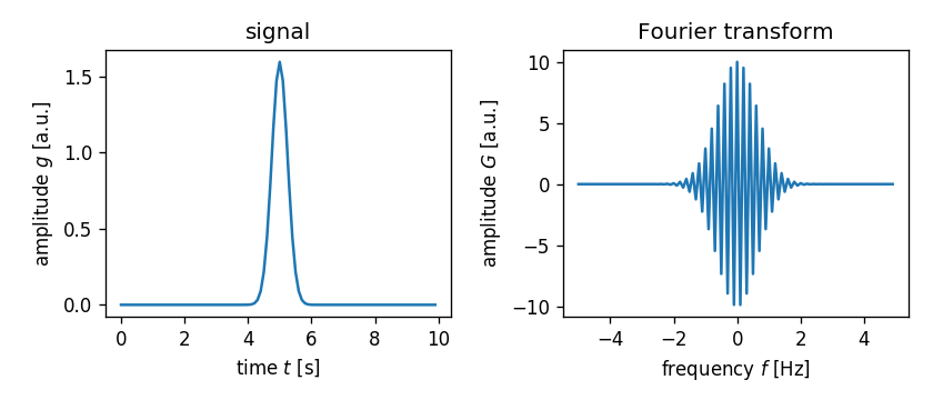
What happened? The Fourier transformed signal rapidly changes signs while
one could only make out a Gaussian envelope. To understand
what went wrong, we need to take a closer look at what numpy.fft.fft
actually does.
First, let us consider the continuous Fourier transform $G(f)$ of a signal $g(t)$,
\[G(f) = \int_{-\infty}^{\infty} g(t) \cdot e^{-2\pi i ft}\,dt.\]In order to discretize this equation, we replace the integral by a sum of $N$ points, forcing us to reduce the integration interval from $(-\infty, \infty)$ to $(0, N)$. Furthermore, we choose the substitutions $f \rightarrow k, k \in \Bbb N$ and $t \rightarrow n/N, n \in \Bbb N$, which leads to the normalization $dt \rightarrow 1$. The discrete signals are now described as $G_k = G(f_k)$ and $g_n = g(t_n)$. The discrete Fourier transform can thus be written as
\[G_k = \sum_{n=0}^{N-1} g_n \cdot e^{-\frac {2\pi i}{N} k n}.\]Note how the definition of $t=0$ has become $n=0$, which brings us back to
the original problem. The origin of $g_k$ is located at $k=0$ (not at
the center of the array $k = N/2$). Thus, in order to get the
Fourier transform of our Gaussian signal right, we would have to shift $g_k$ such
that its maximum is located at $k=0$ (the first element of the array).
We could achieve this by means of np.fft.fftshift, but that only works
as long as the center of $g$ coincides exactly with $n=N/2$.
A more elegant solution is to directly correct for the temporal shift $\tau$
after the Fourier transform. Let’s consider a shifted function $g(t-\tau)$
in the equation of the continuous Fourier transform:
We would like to get rid of the shift $\tau$ and thus substitute $t \rightarrow t + \tau$.
\[G(f) = \int_{-\infty}^{\infty} g(t) \cdot e^{-2\pi i f(t+\tau)}\,dt.\]This step only affects the Fourier kernel and results in the additional term $\exp (- 2 \pi i f \tau)$ which can be pulled out of the integral. This oscillatory term is a simple time shift and explains the artifacts in the figure above. We can correct for this time shift by multiplying $G_k$ with $\exp (+ 2 \pi i f \tau)$:
# correct for time shift `tau`
ft_cor = np.fft.fft(sig) * np.exp(2*np.pi*1j*freq*tau)

fig = plt.figure(figsize=(7, 3))

ax1 = plt.subplot(121, title="signal")
ax1.plot(time, sig)
ax1.set_xlabel("time $t$ [s]")
ax1.set_ylabel("amplitude $g$ [a.u.]")

ax2 = plt.subplot(122, title="time-shift corrected Fourier transform")
ax2.plot(np.fft.fftshift(freq), np.fft.fftshift(ft_cor.real))
ax2.set_xlabel("frequency $f$ [Hz]")
ax2.set_ylabel("amplitude $G$ [a.u.]")

plt.tight_layout()
plt.savefig("shift_corrected.png", dpi=120)
plt.close()
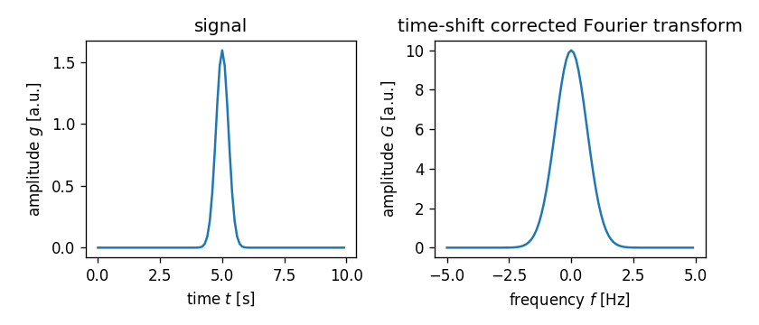
Note that this correction works for any real-valued $\tau$ (as long as the support of $g(t)$ is within the interval $0\,\text{s} < t < 10\,\text{s}$).
Frequency shifting
In some cases, it can be useful to manipulate a signal such that it shows up at a predefined frequency in Fourier space. A frequency shift can be described with
\[G(f-f_0) = \int_{-\infty}^{\infty} g(t) \cdot e^{-2\pi i (f-f_0)t}\,dt.\]In other words, the signal $g(t)$ must be multiplied by the complex exponential $\exp(-2\pi i f_0t)$ to shift its Fourier transform by $f_0$. Here is an example for a shift by 2.2 Hz.
# multiply input with complex exponential
sig_shift = sig * np.exp(2*np.pi*1j*(time-tau)*2.2)
ft_shift = np.fft.fft(sig_shift) * np.exp(2*np.pi*1j*freq*tau)

fig = plt.figure(figsize=(7, 3))

ax1 = plt.subplot(121, title="signal × complex exponential")
ax1.plot(time, sig_shift.real)
ax1.set_xlabel("time $t$ [s]")
ax1.set_ylabel("amplitude $g$ [a.u.]")

ax2 = plt.subplot(122, title="frequency-shifted Fourier transform")
ax2.plot(np.fft.fftshift(freq), np.fft.fftshift(ft_shift.real))
ax2.set_xlabel("frequency $f$ [Hz]")
ax2.set_ylabel("amplitude $G$ [a.u.]")

plt.tight_layout()
plt.savefig("shift_frequency.png", dpi=120)
plt.close()
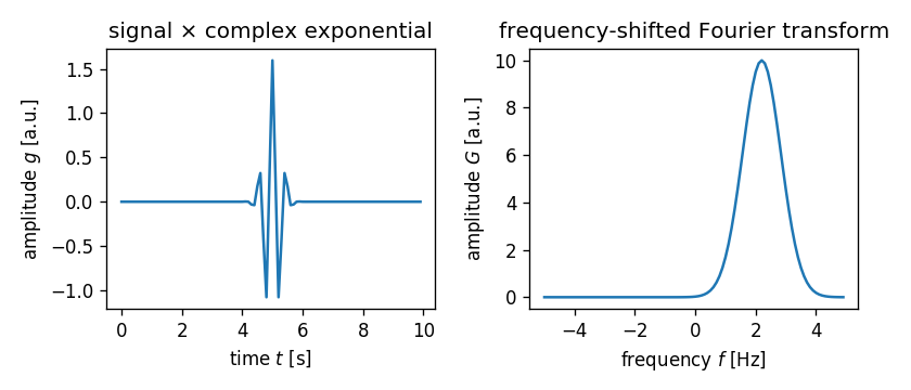
Note again that $\tau$ must be included to correctly shift the
frequency, hence the term time-tau in the complex exponential.
Time scaling
The time scaling property of the Fourier transform states that a change of the sampling frequency in the input signal is equivalent to a scaled signal in Fourier space.
\[\frac{1}{a} G(f/a) = \int_{-\infty}^{\infty} g(at) \cdot e^{-2\pi i f t}\,dt\]In this example, the time axis is scaled by a factor of two, which leads to a Fourier signal that is scaled by a factor of two and narrowed by a factor of one half.
# scale by a factor of 2
freq_sc = np.fft.fftfreq(N, dt/2)

time_sc = time / 2
tau_sc = tau / 2
sig_sc = 1/(sigma * np.sqrt(2*np.pi)) * np.exp(-1/2 *
                                               ((time_sc-tau_sc) / sigma)**2)
ft_sc = np.fft.fft(sig_sc) * np.exp(2*np.pi*1j*freq_sc*tau_sc)
ft_sc = np.fft.fftshift(ft_sc)

freq = np.fft.fftshift(freq)
freq_sc = np.fft.fftshift(freq_sc)

fig = plt.figure(figsize=(7, 3))

ax1 = plt.subplot(121, title="time-scaled signal")
ax1.plot(time, sig_sc.real)
ax1.set_xlabel("time $t$ [s]")
ax1.set_ylabel("amplitude $g$ [a.u.]")

ax2 = plt.subplot(122, title="scaled Fourier transform")
ax2.plot(freq, ft_sc.real)
ax2.set_xlabel("frequency $f$ [Hz]")
ax2.set_ylabel("amplitude $G$ [a.u.]")

plt.tight_layout()
plt.savefig("scale_time.png", dpi=120)
plt.close()
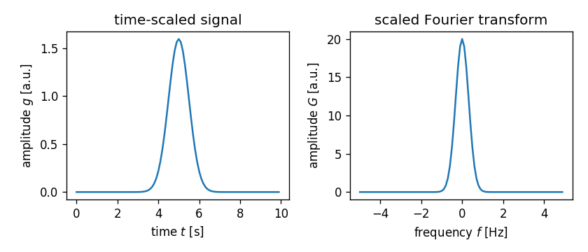
Image translation
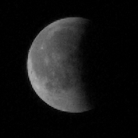
Many applications of the Fourier transform involve image analysis. It is possible to perform the trivial task of image translation with the Fourier transform. If the image is translated by a non-integer amount of pixels, then the interpolation takes place with the Fourier kernel (sine and cosine functions). For this example, we use a downscaled image of the lunar eclipse, recorded on July 27th 2018.
import matplotlib.image as mpimg

moon = mpimg.imread("moon_small.png")
fy = np.fft.fftfreq(moon.shape[0]).reshape(-1, 1)
fx = np.fft.fftfreq(moon.shape[1]).reshape(1, -1)
ft_moon = np.fft.fft2(moon) * np.exp(2*np.pi*1j*(fx*10.5 + fy*10))
moon_tr = np.fft.ifft2(ft_moon)

fig = plt.figure(figsize=(7, 3.6))

ax1 = plt.subplot(121, title="moon")
ax1.imshow(moon, cmap="gray", interpolation="none")

ax2 = plt.subplot(122, title="translated moon")
ax2.imshow(moon_tr.real, cmap="gray", interpolation="none")

plt.tight_layout()
plt.savefig("moon_translated.png", dpi=120)
plt.close()
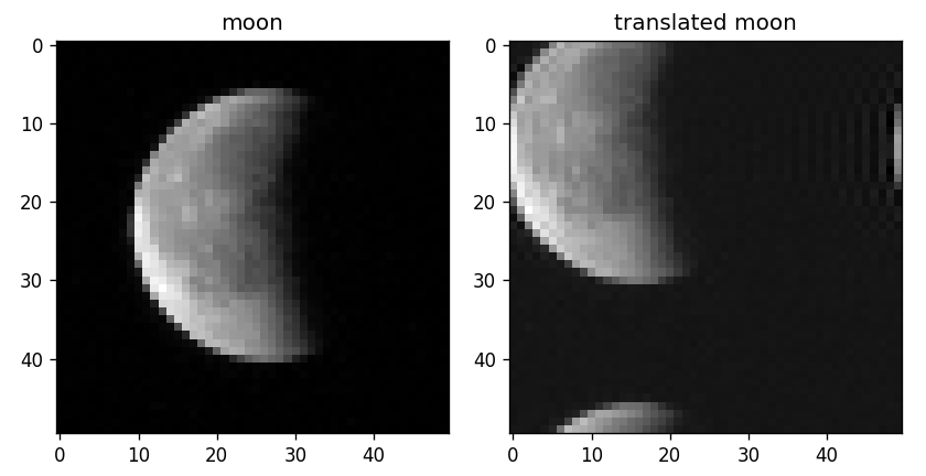
The image is translated by 10 pixels along the y-axis and by 10.5 pixels along the x-axis. The resulting interpolation along the x-axis leads to horizontal ringing artifacts.
Performing image translation with the Fourier transform might be fast, but for higher accuracy, other interpolation methods (e.g. splines) might be better suited, especially when sharp boundaries (dark-bright) are present.
Image modulation: Holograms
The Fourier transform can be used for the analysis of digital holograms. In the life sciences, digital holographic imaging is used to quantify the refractive index of cells. To achieve that, a laser beam is split into two beams, one passes through the sample and the other serves as a reference. When these two beams are brought back together at a slightly tilted angle, they generate an interference pattern, periodic stripes that can be recorded with a regular camera, that is modulated by the phase delay introduced by the varying refractive index of the sample.
The example hologram shows an HL60 cell - the intensity data clearly reveals a cell, but we are after the phase data. The modulation of the phase data becomes visible when tracing the interference pattern (dark stripes) through the cell: they appear to be deformed at the cell boundary. This modulation can be extracted with Fourier analysis. The interference pattern can be described as a cosine function, whose Fourier transform are two delta functions, the so-called sidebands. Isolating one of those sidebands (see arrow in the image below) and performing an inverse Fourier transform, reveals the part of the light that passed through the cell and the phase delay can be computed.
cell = mpimg.imread("cell_hologram.png")
ft_cell = np.fft.fft2(cell)
ft_cell_copy = np.copy(ft_cell)
# suppress central band
ft_cell[0, :] = 0
ft_cell[:, 0] = 0
# determine sideband position
xmax = np.argmax(np.max(ft_cell, axis=1))
ymax = np.argmax(ft_cell[xmax])

# move sideband to zero frequency
ft_cell_rolled = np.roll(ft_cell, (-xmax, -ymax), axis=(0, 1))
# apply sideband filter
ft_cell_rolled[20:-20, :] = 0
ft_cell_rolled[:, 20:-20] = 0
# invert to get sideband modulation
modulation = np.fft.ifft2(ft_cell_rolled)
# compute phase
phase = np.angle(modulation)

fig = plt.figure(figsize=(7, 2.8))

ax1 = plt.subplot(131, title="hologram")
ax1.imshow(cell.real, cmap="gray", interpolation="bilinear")

ax2 = plt.subplot(132, title="Fourier transform")
ax2.imshow(np.fft.fftshift(np.log(1 + np.abs(ft_cell_copy))),
           interpolation="none")
ax2.arrow(37, 50, 32, 11, head_length=10, head_width=10, fc='w', ec='w')
ax3 = plt.subplot(133, title="wrapped phase")
ax3.imshow(phase, cmap="coolwarm", interpolation="none")

for ax in [ax1, ax2, ax3]:
    ax.set_xticks([])
    ax.set_yticks([])

plt.tight_layout(w_pad=0, pad=0, h_pad=0)
plt.savefig("cell_modulation.png", dpi=120)
plt.close()
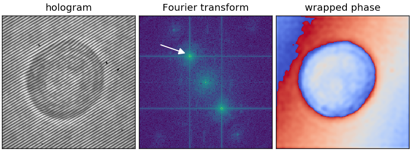
Note that the phase is wrapped in the interval $(0, 2\pi)$, i.e. there are $2\pi$ phase jumps (from red to blue) that have to be “unwrapped” for further analysis.
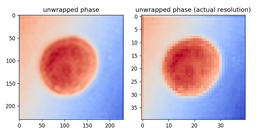
Scaling images
The Fourier transform can also be used to up- or downscale images. In the above example, the inverse Fourier transform was performed for a much larger frequency space than necessary, because we actually cropped the sideband to 40 by 40 pixels. If we only take the inverse Fourier transform of the cropped sideband, we get an idea of the actual image resolution. In short, upscaling with the Fourier transform means that the image is interpolated with cosine functions. On the other hand, downscaling with the Fourier transform means that high-frequency contributions are omitted. The illustration below additionally makes use of a phase unwrapping algorithm that is part of the scikit-image library.
from skimage.restoration import unwrap_phase

ft_cell_low = np.zeros((40, 40), dtype=complex)
ft_cell_low.flat[:] = ft_cell_rolled[ft_cell_rolled != 0]
modulation_low = np.fft.ifft2(ft_cell_low)
# compute phase
phase_low = unwrap_phase(np.angle(modulation_low))
phase = unwrap_phase(phase)

fig = plt.figure(figsize=(7, 3.6))

ax1 = plt.subplot(121, title="unwrapped phase")
ax1.imshow(phase, cmap="coolwarm", interpolation="none")

ax2 = plt.subplot(122, title="unwrapped phase (actual resolution)")
ax2.imshow(phase_low, cmap="coolwarm", interpolation="none")

plt.tight_layout()
plt.savefig("cell_downsampled.png", dpi=120)
plt.close()
Watermarks
A watermark is a modification of an image, often used to prevent (or track) the usage of an image by others. Watermarks are usually just image overlays, but they can also be hidden in Fourier space. Note that the modification in Fourier space results in distortions, present everywhere in the image, whose intensity depends on the number of frequencies used and the corresponding amplitudes. In this example, an image of the lunar eclipse is watermarked with a smiley.
moon = mpimg.imread("moon.png")
fy = np.fft.fftfreq(moon.shape[0]).reshape(-1, 1)
fx = np.fft.fftfreq(moon.shape[1]).reshape(1, -1)
ft_moon = np.fft.fft2(moon)
smile = mpimg.imread("smile.png")
smile_pad = np.zeros_like(moon, dtype=complex)
smile_pad[-(20+smile.shape[0]):-20, -(60+smile.shape[1]):-60] = smile
moon_mark = np.fft.ifft2(ft_moon + 10*smile_pad)
ft_mark = np.fft.fft2(moon_mark.real)

fig = plt.figure(figsize=(7, 2.8))

ax1 = plt.subplot(131, title="moon")
ax1.imshow(moon, cmap="gray", interpolation="none")

ax2 = plt.subplot(132, title="watermarked moon")
ax2.imshow(moon_mark.real, cmap="gray", interpolation="none")

ax3 = plt.subplot(133, title="Fourier transform")
ax3.imshow(np.log(1 + np.abs(np.fft.fftshift(ft_mark))), interpolation="none")
ax3.arrow(55, 30, -15, 15, head_length=8, head_width=8, fc='w', ec='w')

for ax in [ax1, ax2, ax3]:
    ax.set_xticks([])
    ax.set_yticks([])

plt.tight_layout(w_pad=0, pad=0, h_pad=0)
plt.savefig("moon_watermark.png", dpi=120)
plt.close()
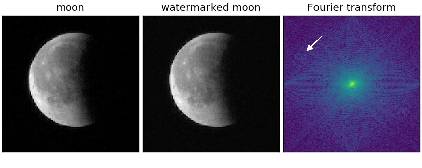
Note that watermarks may also cover only a few pixels in Fourier space which are then not as easily spotted as in the example above. Also note that depending on the used frequencies of the watermark, scaling down the image might or might not remove the watermark.